neo_mpc_planner

The Model Predictive Control (MPC) is an optimization-based feedback control technique, which was initially developed for the field of process industries. With the recent advancements in cost-effective computation, MPC was extended to the field of robotics for real-time control. This means that the optimization happens on the fly. MPC otherwise also called Receding Horizon Control (RHC) is utilized in robots for path following and/or trajectory tracking.

neo_mpc_planner2 is exclusively developed for quasi-omnidirectional robots such as Neobotix MPO-700, but can also be used on mecanum-wheeled robots such as Neobotix MPO-500. MPO-700 is used for transporting various objects in a structured environment. Therefore this planner aims in catering to all the omni-directional robots used in a known environment. The controller was tested on an Intel i5 processor and was found that it can easily work at an average rate of 50 Hz. This would help to instantaneously react to suddenly occurring obstacles. Currently, the planner is designed in a way to stop the robot if there is an unknown obstacle in the predicted path.

The entire planner is built on the Navigation2 stack for ROS 2. Currently, the planner supports omni-directional robots only and later it will be extended to differential robots.

Background on MPC

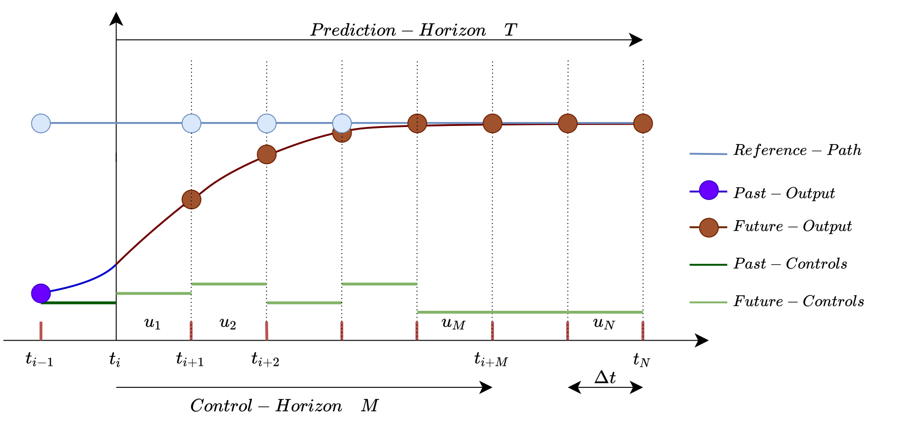
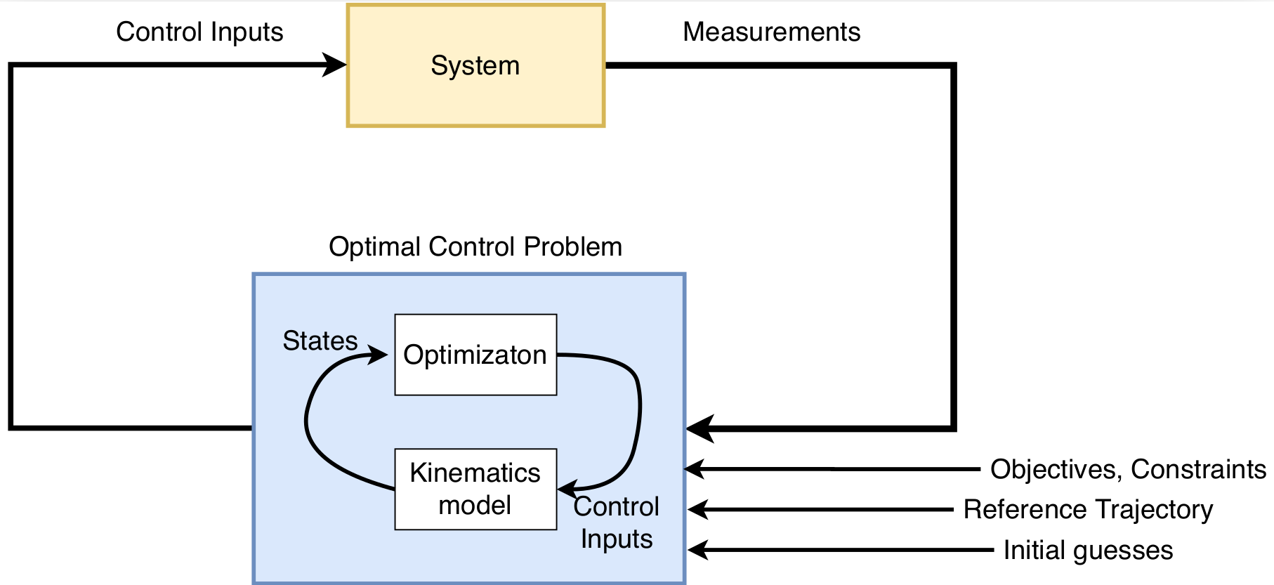
The above figure depicts a brief overview of the evolution of MPC. The control architecture of an MPC consists of an empirical model of the system and optimal control, which provides feedback resulting in a closed-loop system. MPC determines the future output by generating the control steps from the current time \(t_i\). The control steps (\(u_1, u_2, ..., u_N\)) are identified by solving an open-loop Optimal Control Problem (OCP) during a specific prediction horizon T with the current state as the initial state. The number of control steps N is pre-defined. Control horizon M represents the time period \(t_{i+M}\) up to which the control steps are found, and beyond which the controls are held constant. Therefore, the prediction horizon will always be greater than or equal to the control horizon. ∆t represents the interval between the two successive control steps and the value of this is determined by finding the ratio of the prediction horizon and the number of control steps. The optimal control problem takes into account the associated constraints with the system. Solving the OCP for particular control horizon yields the necessary control steps for the system to be able to evolve. The first generated control step is applied to the system, which results in a shift in the system’s position. Again the entire process is repeated until the system reaches the final desired state. In most cases, the OCP is warm-started with the remaining updates from the prior optimization process being employed as the initial guesses. By utilizing the states as feedback at every step, the controller can reject unnecessary disturbances or deviations caused by the system model. The control diagram of the MPC is seen below.

There are different methods to solve OCP, which will not be further discussed in this article. The method to solve OCP for this particular algorithm is known as the single-shooting approach.

Every controller out there has a path-following strategy. For MPC, it was decided to apply the pure-pursuit method for following the path.

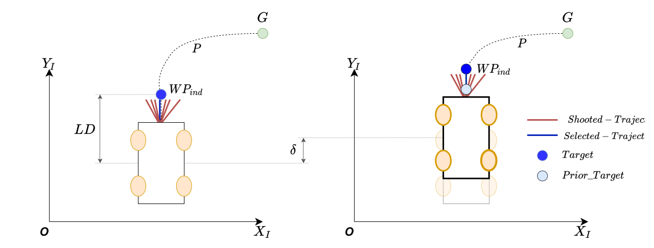
A lookahead distance LD is defined at the initialization. Depending on the LD, the waypoint is selected on the given path. For this particular package, it is the global planner. Once the MPC starts applying the velocity commands, lookahead point is moved depending on the distance the robot has travelled. In any case, the lookahead distance is always kept constant.

With all the above information, below we discuss the generation of velocity commands for a single control step. The process involved is as follows:

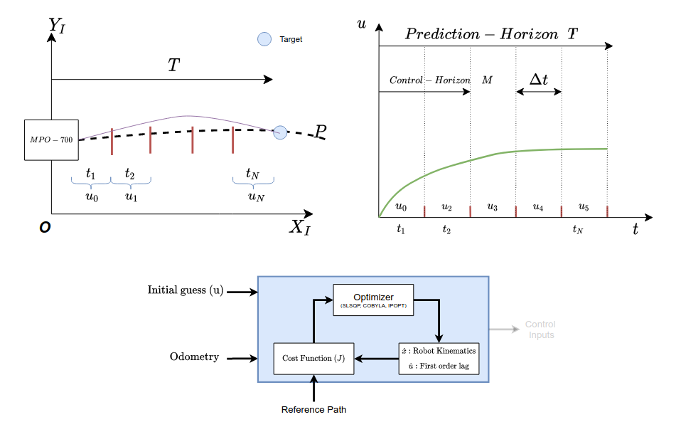
Assume that a robot is placed in a known environment, as shown below.

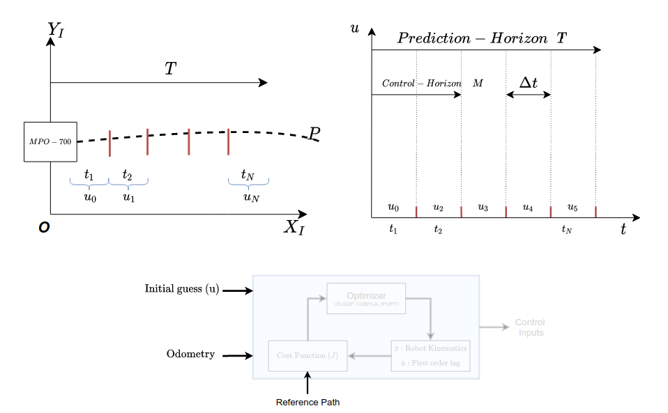
As seen in the figure, it can be noted a Prediction horizon T and the number of control steps N has been defined. Also since it is known that it is an optimization-based algorithm, it requires initial guesses for the control steps. The initial guesses here are the (\(u_0, u_1, ..., u_N\)), which are discretized based on the control steps N. An Ordinary Differential Equation (ODE) consisting of the prediction model is considered an initial value problem and is solved for the same. On solving the initial value problem, control steps are yielded as shown below.

The optimizer generates multiple trajectories and selects the lowest cost trajectory as shown in the image below. The controller then applies the first control step. Note that, the prediction model of the system is nothing but the kinematics of the system.

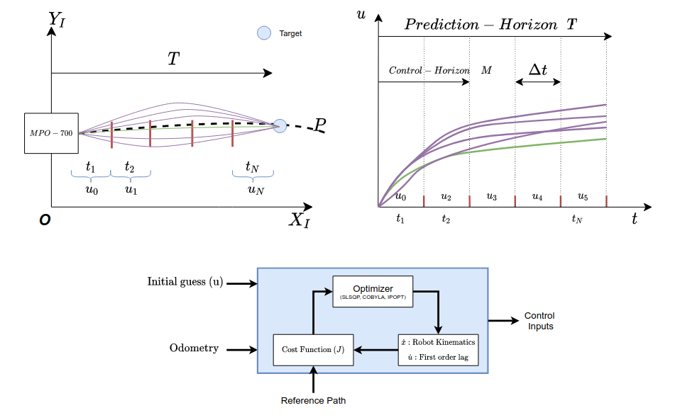
The entire process is repeated, with the optimizer being warm-started from the outputs generated by the previous step as the initial guess. This process is repeated until the robot reaches the user-specified goal location

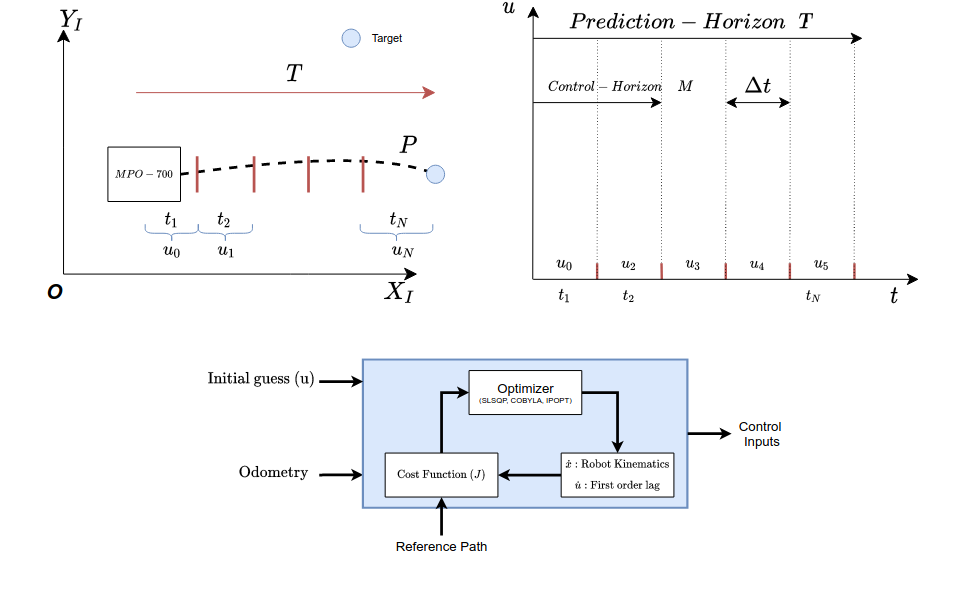
The odometry data is utilized in the cost function to determine the deviation from the lookahead point and as well the goal location.

Tuning guide

ToDo

Further reading

ToDo